Plotting

In this section we’ll cover some of main plotting functionality within HAWKS. For full documentation of the plotting functions, see hawks.plotting.

As with the Examples, the images and code shown here are demonstrative and are not intended to show actual research.

Instance space

For visualizing the datasets according to their problem features (or meta-features), we can plot the instance space. PCA is used to reduce the problem features down to 2D. For more about instance spaces, see our paper, or e.g. this work.

"""This example shows a quick instance space for some uninteresting datasets from HAWKS and :mod:`sklearn.datasets`.
"""
from sklearn.datasets import make_blobs, make_moons
import seaborn as sns

import hawks

SEED_NUM = 10
NUM_RUNS = 10 # May take a few minutes
NUM_CLUSTERS = 5

generator = hawks.create_generator({
    "hawks": {
        "seed_num": SEED_NUM,
        "num_runs": int(NUM_RUNS/2) # for parity
    },
    "dataset": {
        "num_clusters": NUM_CLUSTERS
    },
    "objectives": {
        "silhouette": {
            "target": [0.5, 0.9]
        }
    }
})
generator.run()
# Analyse the hawks datasets
df, _ = hawks.analysis.analyse_datasets(
    generator=generator,
    source="HAWKS",
    seed=SEED_NUM,
    save=False
)
# Make the blobs datasets
datasets = []
label_sets = []
for run in range(NUM_RUNS):
    data, labels = make_blobs(
        n_samples=1000,
        n_features=2,
        centers=NUM_CLUSTERS,
        random_state=SEED_NUM+run
    )
    datasets.append(data)
    label_sets.append(labels)
# Analyse the blobs datasets
df, _ = hawks.analysis.analyse_datasets(
    datasets=datasets,
    label_sets=label_sets,
    source="SK-Blobs",
    seed=SEED_NUM,
    save=False,
    prev_df=df
)
# Make the moons datasets
datasets = []
label_sets = []
for run in range(NUM_RUNS):
    data, labels = make_moons(
        n_samples=1000,
        noise=2,
        random_state=SEED_NUM+run
    )
    datasets.append(data)
    label_sets.append(labels)
# Analyse the moons datasets
df, _ = hawks.analysis.analyse_datasets(
    datasets=datasets,
    label_sets=label_sets,
    source="SK-Moons",
    seed=SEED_NUM,
    save=False,
    prev_df=df
)
# Make the font etc. larger
sns.set_context("talk")
# Make the boxplot
hawks.plotting.instance_space(
    df=df,
    color_highlight="source",
    marker_highlight="source",
    show=True,
    seed=SEED_NUM,
    cmap=sns.cubehelix_palette(3)
)

Output:

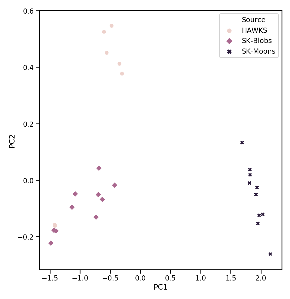
The instance space of the three sets of datasets.

Visualizing convergence

AS HAWKS is underpinned by an evolutionary algorithm, it’s useful to be able to visualize convergence of the algorithm to better understand the optimization. For this, hawks.plotting.convergence_plot() provides a general function for plotting this. By default, the fitness is used for the y-axis, though this can be controlled by the y argument (as long as it matches a column in the stats DataFrame).

"""This example demonstrates generating convergence plots for the fitness and overlap (constraint).
"""
import seaborn as sns

import hawks

# Create the generator
generator = hawks.create_generator({
    "hawks": {
        "seed_num": 42,
        "num_runs": 5
    },
    "dataset": {
        "num_clusters": 5
    },
    "objectives": {
        "silhouette": {
            "target": 0.9
        }
    },
    "constraints": {
        "overlap": {
            "threshold": 0.05,
            "limit": "lower"
        }
    }
})
# Run HAWKS!
generator.run()
# Make a dictionary of options common to both plots
converg_kws = dict(
    show=True,
    xlabel="Generation",
    ci="sd",
    legend_type=None
)
# Make the font etc. larger
sns.set_context("talk")
# Plot the fitness (proximity to silhouette width target)
hawks.plotting.convergence_plot(
    generator.stats,
    y="fitness_silhouette",
    ylabel="Average Fitness",
    clean_props={
        "legend_loc": "center left"
    },
    **converg_kws
)
# Plot the overlap constraint
hawks.plotting.convergence_plot(
    generator.stats,
    y="overlap",
    clean_props={
        "clean_labels": True, # Capitalize the 'overlap' y-axis label
        "legend_loc": "center left"
    },
    **converg_kws
)

Output:

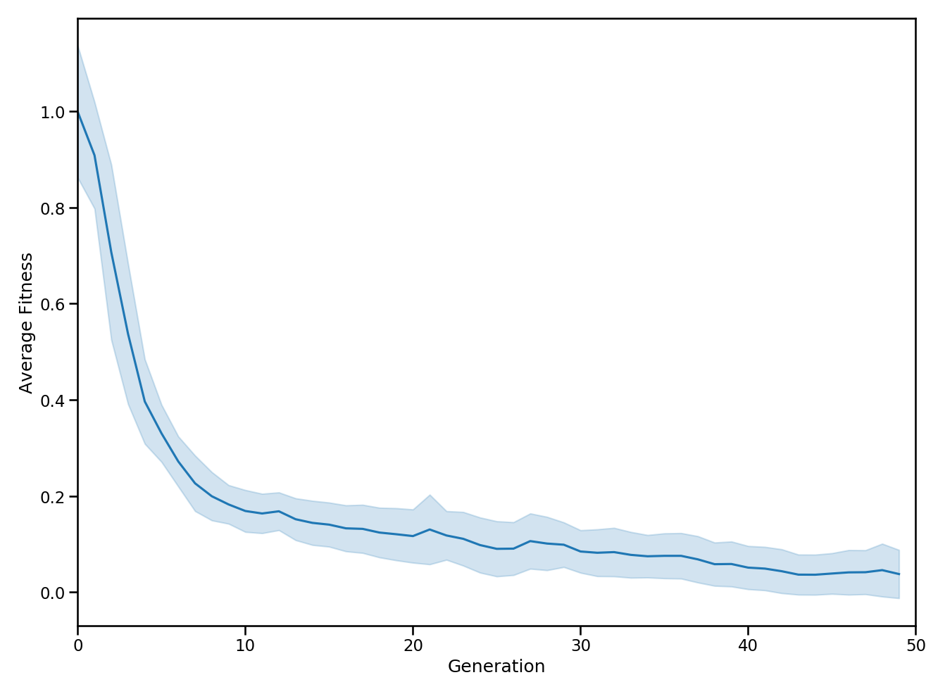
Convergence of the fitness

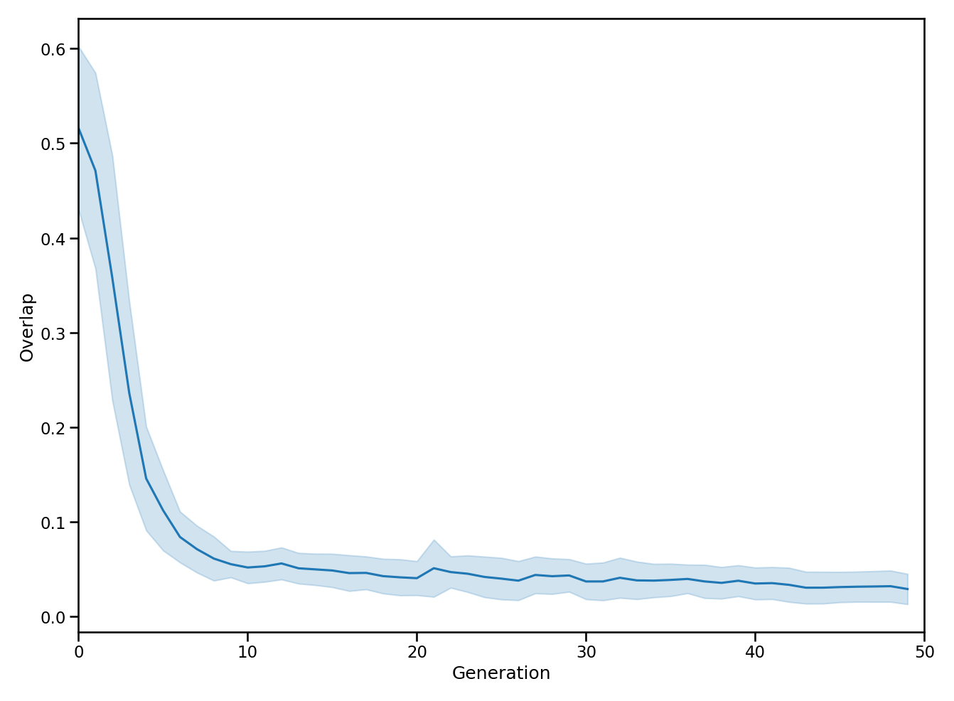
Convergence of the overlap

Todo

Add further examples.